Receiver Operating Characteristic (ROC) Plot
metric: dprime, aprime, amzs (default is dprime)
isopleths: None, beta, c, bppd, bmz
fname: outputname
dpi: resolution of plot
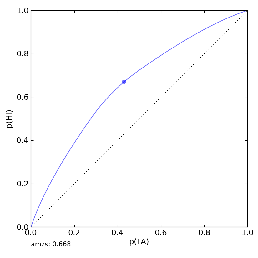
ROC plots can be generated from dprime, aprime, or amzs
>>> from sdt_metrics.plotting import roc_plot
>>> roc_plot(.67, .43, metric='amzs', fname='roc_example01.png')
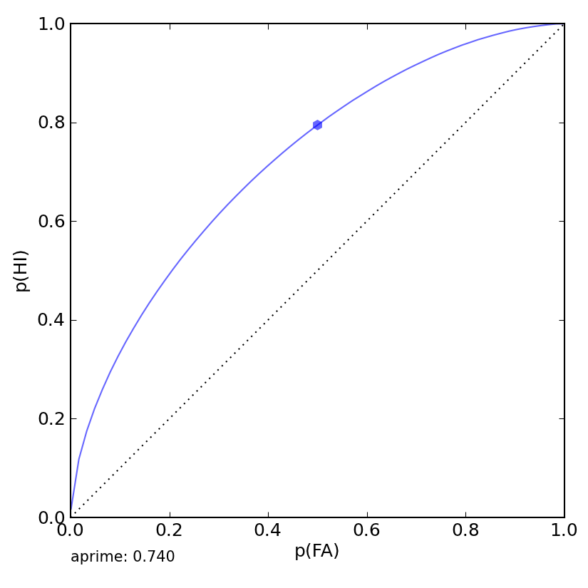
>>> roc_plot(116, 30, 50, 50,
             metric='aprime',
             fname='roc_example02.png')
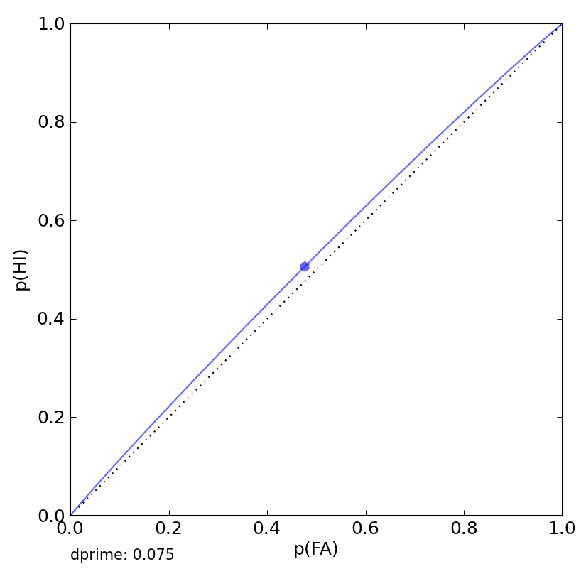
>>> from sdt_metrics import HI,MI,CR,FA, SDT
>>> from random import choice
>>> sdt_obj = SDT([choice([HI,MI,CR,FA]) for i in xrange(1000)])
>>> print(sdt_obj)
SDT(HI=251, MI=245, CR=264, FA=240)
>>> roc_plot(sdt_obj, fname='roc_example03.png')
The isopleths keyword allows specifying isopleths for either beta, c, bppd, or bmz.
>>> roc_plot(116, 30, 50, 50,
             metric='dprime',
             isopleths='beta',
             fname='roc_example04.png')
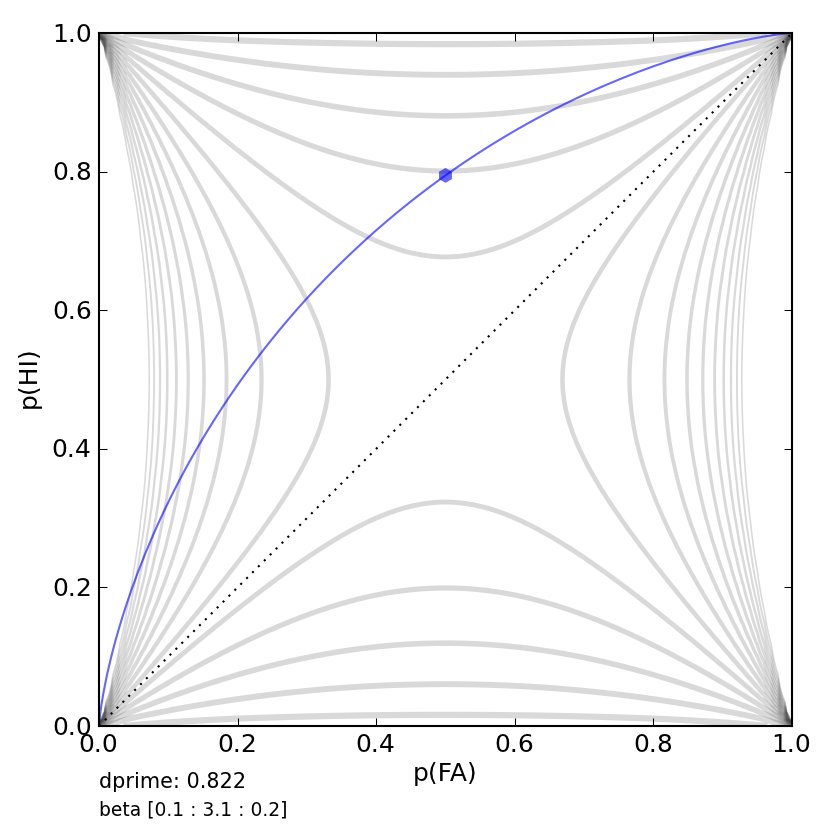
The values inside the brackets specify [start : stop : step]. On The figure the thinner lines denot larger values (going up hill). This is a little counterintuitive but the uphill gradients tend to be steeper and having thinner lines makes the plots look better.