
B’‘D is generally acknowledged as being the preferred and robust nonparametric measure of decision bias. Despite its popularity, B’‘D has an Achilles’ heel with boundary cases where it loses sensitivity. Applying a loglinear transform to B’‘D fixes the boundary cases and is otherwise benign.
When the parametric assumptions of c do not hold a nonparametric alternative is needed. In the literature a multitude of measures are available, including but not limited to: B’H, B’‘, B’‘d, and B_MZ [SEE1997], [HODOS1970], [GRIER1971], [DONALDSON1992], [ZHANG2005]. Of these B’‘d is the most highly recommended [SEE1997], [SZALMA]. It?s creator and origins stem from memory recognition research [DONALDSON1992], and subsequent theoretical and empirical comparisons have shown it to be robust in vigilance settings [SEE1997] and that it yields accurate estimates when data is collapsed or grouped [MACMILLAN1990] and [SNODGRASS1998] (secondary citation from [SEE1997]).
B’‘d is calculated from hit and false alarm rates and is well behaved over most of its domain. The exception being at the hit and false alarm rates boundaries B’‘d loses sensitivity. The plot below depicts B’‘d versus c. The 121 points reflect factorial combinations of hit rates between 0 and 1 at .1 increments and false alarm rates between 0 and 1 at .1 increments.
.png)
Examing how B’‘d is computed reveals some insight into this phenomena. B’‘d is a function of pHI and pFA (hit rate and false alarm rate respectively),
                  (1-pHI)(1-pFA) - pHI*pFA
B''D(pHI, pFA) = --------------------------
                  (1-pHI)(1-pFA) + pHI*pFA

    where,
       pHI = HI/(HI+MI)
       pFA = FA/(FA+CR)
Losses of sensitivity occur on the boundaries. B’‘D always yields 1 when:
                              (1-pFA)
B''D(pHI = 0, 0 < pFA < 1) = ---------
                              (1-pFA)
Regardless of the actually false alarm rate B’‘D yields 1. A valid measure of response bias should correlate with the false alarm rate under these circumstances. B’‘D is also 1 when:
                              (1-pHI)
B''D(pFA = 0, 0 < pHI < 1) = ---------
                              (1-pHI)
On the other boundaries B’‘D always becomes -1,
                              -pFA
B''D(pHI = 1, 0 < pFA < 1) = ------
                               pFA
and when,
                              -pHI
B''D(pFA = 1, 0 < pHI < 1) = ------
                               pHI
Here a correction to B’‘D is suggested. When calculating d? a common treatment of extreme values is to apply a loglinear transformation to the hit rate and false alarm rates [HAUTUS1995]. The transformation calculates hit rate as,
pHI = (HI+0.5)/(HI+MI+1)
and the false alarm rate as,
pFA = (FA+0.5)/(FA+CR+1)
The effect is that the rates are compressed but maintain interval scaling. The loglinear corrected values of d’ will always be of slightly lower magnitude due to the compression but the result is a well accepted measure of sensitivity. Similar treatments also apply to beta and c. Here, I suggest the loglinear transformation can be applied to B’‘D to correct the boundary condition problems describe above and the consequences to non-boundary values of pHI and pFA are negligible.
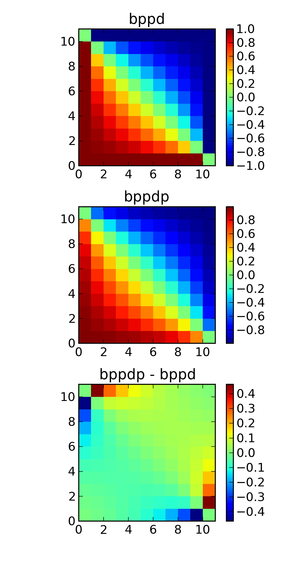
The following scatter matrix demonstrates how the loglinear transformation corrects the boundary of B’‘D. It also demonstrates that over most of its range B’‘D (bppd) and the loglinear B’‘D (loglinear_bppd) are highly correlated.
.png)
Applying the transformation alleviates the boundary sensitivity problems. Examining bppd and loglinear_bppd in ROC space provides further reassurance.

The x and y axes are showing false alarm counts and hit counts respectively.
As suggested by the above figures bppd and loglinear_bppd are highly correlated.
The plot below depicts cases where the boundary conditions are excluded.
.png)
When the prevalence rate drops from chance to 10% (5 true events, 45 false events) the correlation between bppd and loglinear_bppd yields an R^2 of .9910 across the non-boundary cases.
.png)
The new measure asymptotically approaches -1 when the observed hit rate is 1 and the observed false alarm rate is 1 as the number of events increases, and asymptotically approaches 1 when the observed hit rate is 0 and the observed false alarm rate is 0.
                   /     1             1      \
max(|B''D|) = B''D| ------------, ------------ |
                   \ 2(HI+MI+1)    2(FA+CR+1) /
.png)
When the prevalence rate is 50% the response bias is as expected to an observed hit rate of 1 and false alarm rate of 0 is the prevalence rate shifts from 50% the response bias also shifts:
>>>             #  HI, MI, CR, FA
>>> loglinear_bppd(10, 0,  10,  0)
-3.9981245827275e-16
>>> loglinear_bppd(10, 0,  11,  0)
0.045454545454545026
>>> loglinear_bppd(10, 0,  12,  0)
0.08695652173912993
>>> loglinear_bppd(10, 0,  13,  0)
0.12499999999999958
>>> loglinear_bppd(10, 0,  14,  0)
0.15999999999999956
The loglinear transformed false alarm rates decrease in proportion to the loglinear hit rate the bias shifts quite quickly because the isopleths in this region of ROC space are particularly steep. A similiar shift occurs when the hit observed hit rate is 0 and the observed false alarm rate is 1.
This also occurs with loglinear_c although the isopleths are not quite as problematic:
>>>          #  HI, MI, CR, FA
>>> loglinear_c(10,  0, 10,  0)
-1.0436096431476471e-14
>>> loglinear_c(10,  0, 11,  0)
0.020521384119198904
>>> loglinear_c(10,  0, 12,  0)
0.0391017058301415
>>> loglinear_c(10,  0, 13,  0)
0.056060731747756054
>>> loglinear_c(10,  0, 14,  0)
0.07164650351337443
Sometimes the distinction between a bug and a feature is in the documentation.
| [DONALDSON1992] | (1, 2) Donaldson, W. (1992). Measuring recognition memory. Journal of Experimental Psychology: General, 121, 275277. |
| [GRIER1971] | Grier, J. B. (1971). Nonparametric indexes for sensitivity and bias: Computing formulas. Psychological Bulletin, 75, 424-429. |
| [HAUTUS1995] |
| [HODOS1970] | Hodos, W. (1970). A nonparametric index of response bias for use in detection and recognition experiments. Psychological Bulletin, 74, 351-354. |
| [MACMILLAN1990] | Macmillan, N. A., and Creelman, C. D. (1990). Response bias: Characteristics of detection theory, threshold theory, and “nonparametric” indexes. Psychological Bulletin, 107, 401- 413. |
| [SEE1997] | (1, 2, 3, 4) See, J. E., Warm, J. S., Dember, W. N., and Howe, S. R. (1997). Vigilance and signal detection theory: An empirical evaluation of five measures of response bias. |
| [SNODGRASS1998] | Snodgrass, J. G., & Corwin, J. (1988). Pragmatics of measuring recognition memory: Applications to dementia and amnesia. Journal of Experimental Psychology: General, 117, 34-50. |
| [SZALMA] | Szalma, J. L., and Hancock, P. A. Signal detection theory. Class Lecture Notes. http://bit.ly/KIyKkt |
| [ZHANG2005] | Zhang, J., and Mueller, S. T. (2005). A note on roc analysis and non-parametric estimate of sensitivity. Psychometrika, 70, 145-154. |